NIG

In most, if not all, IoT deployments, data needs to be processed, stored, and made consumable or presentable. As discussed in the previous chapter, MQTT provides a way to communicate and transport data between devices and applications. However, after the data is received, it still needs to be processed, stored, and presented.

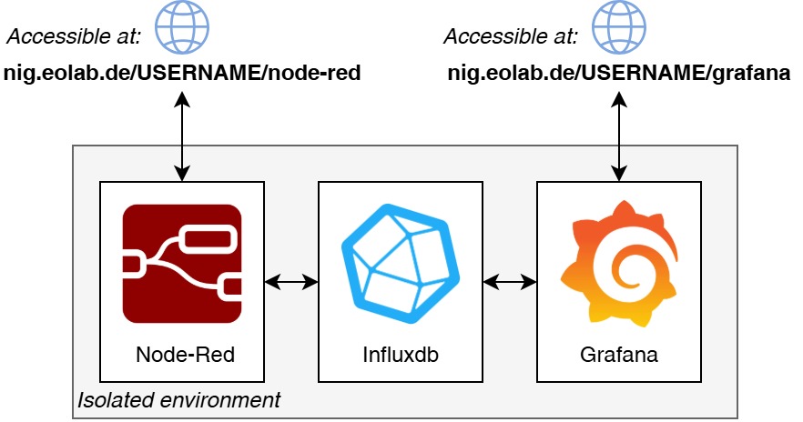
There is no single, universally defined way to achieve this. Each project, company, research group, or institution may have its own tools and processes in place. In AMC, we introduce a toolset called the NIG stack. NIG stands for Node-RED, InfluxDB, and Grafana. The name is a made-up acronym created in the EOLab at HSRW by Jan Sonntag to refer to this combination of tools.

NIG stack.

These tools are individual software components that can operate independently and can be used in a wide variety of industries and projects. At the same time, they provide a high level of integration. When combined, they form an interesting and practical, although not necessarily perfect, toolset for developing IoT applications. More importantly, the NIG stack allows you, as a student, to explore tools that can also be used outside AMC. They can be applied in multiple contexts and can expand your technical toolbox.

We selected the NIG stack because it provides a clean and easy-to-understand separation of concerns:

• Node-RED is used for data processing and integration.
• InfluxDB is used for storing time-series data.
• Grafana is used for presenting data through dashboards.

The stack also provides low-code and no-code approaches for handling parts of an IoT deployment. This is an important capability in AMC, especially because many AMC students come from environmental and energy-related study programs.

Programming, databases, and dashboards can initially sound intimidating or appear to be topics reserved for computer-science specialists. However, the NIG stack reduces much of the implementation overhead and makes these tools more accessible to students without a computer-science background. This does not mean that no technical understanding is required. You still need to understand how data moves through the system, how it is processed, how it is stored, and how it should be presented. The NIG stack allows you to focus on these concepts without having to implement every component from the beginning.

Allow us to present:

Node-RED is a low-code, flow-based programming environment designed to connect hardware devices, communication protocols, databases, APIs, and online services. Applications are created visually by linking functional blocks, called nodes, into a flow. Each node performs a specific task, such as receiving data, transforming a value, applying a condition, storing information, or sending a command to another device. Because the structure of the application is represented graphically, Node-RED makes complex data flows easier to understand, develop, and modify.

InfluxDB is a time-series database designed to store and manage data that changes over time. Unlike conventional relational databases, which organize information mainly into tables and relationships, InfluxDB is optimized for measurements associated with timestamps. Each stored data point can contain a measurement name, one or more field values, identifying tags, and a timestamp. This structure makes InfluxDB particularly suitable for continuously generated data such as sensor readings, system metrics, equipment states, and environmental measurements.

Grafana is a visualization and monitoring platform used to create interactive dashboards from data stored in external data sources. It does not normally store sensor data itself. Instead, it connects to databases and monitoring systems, retrieves the required information, and presents it through visual elements such as graphs, gauges, tables, status indicators, and statistical panels. Dashboards can be configured to display real-time information as well as historical data from a selected time interval.

An additional advantage of the NIG stack is that all three components are open-source software. This allows you to host and manage your own instances.

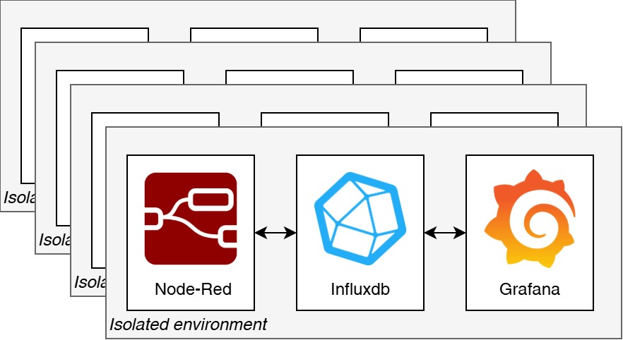
For convenience, however, the AMC Teaching Team provides the infrastructure required for this course. Each student receives an isolated NIG environment containing their own instances of Node-RED, InfluxDB, and Grafana.

NIG stack deployment. Each student and team receives an isolated environment containing dedicated Node-RED, InfluxDB, and Grafana instances.

Only Node-RED and Grafana are directly accessible through the internet. This is intentional. Node-RED provides the interface for processing and writing data, while Grafana provides the interface for reading and presenting it. InfluxDB operates as the internal storage layer between them, so there is normally no need to access it directly in the same way as the other two applications.

In the following sections, you will first become familiar with Node-RED, InfluxDB, and Grafana individually. You will then connect them to create a complete IoT data pipeline: receiving and processing data, storing it, and presenting it in a dashboard.

---

Node-Red

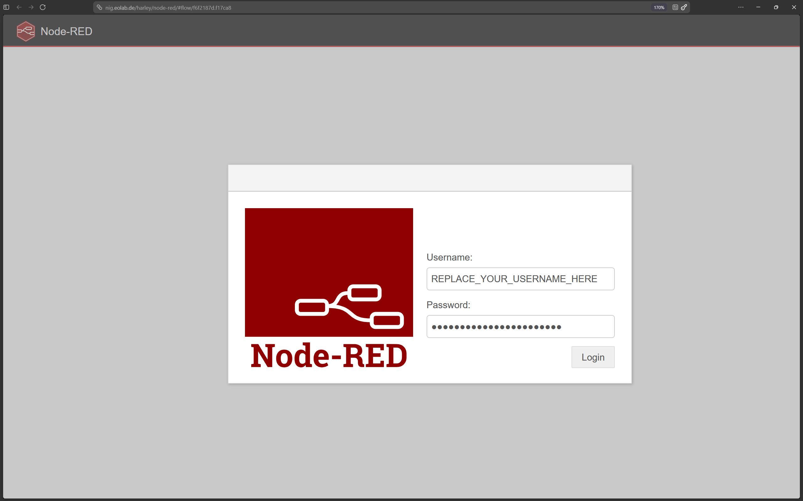
Open your personal Node-RED instance using the URL below. Replace REPLACE_YOUR_USERNAME_HERE with your AMC NIG username before opening it in a browser.

https://nig.eolab.de/REPLACE_YOUR_USERNAME_HERE/node-red

Node-RED sign-in page. Sign in with your AMC NIG account to open the Node-RED editor.

Node-RED is particularly important in Internet of Things applications because it can act as an intermediary between physical devices and software systems. IoT devices continuously generate measurements from sensors, including temperature, humidity, pressure, light, motion, and air-quality data. Node-RED can receive these measurements through protocols such as MQTT, HTTP, WebSockets, or serial communication and then process them before they are stored or displayed. Sensor-data processing may include filtering invalid values, converting units, adding timestamps, calculating averages, combining readings from multiple sensors, and comparing values against predefined thresholds. Based on the processed data, Node-RED can also generate alerts or send control commands to actuators such as fans, pumps, relays, and motors.

Another major advantage of Node-RED is its extensibility and its ability to integrate different technologies within a single application. Its functionality can be expanded by installing additional nodes for specific devices, protocols, databases, cloud platforms, and visualization systems. Node-RED can therefore connect IoT devices with services such as MQTT brokers, REST APIs, SQL or time-series databases, dashboards, cloud platforms, and external applications. When the available nodes are not sufficient, custom processing logic can also be implemented using JavaScript. This flexibility makes Node-RED suitable for rapid prototyping, laboratory experiments, and the development of complete IoT data pipelines.

In the context of the AMC course, Node-RED is used as an interface between the MQTT communication system, the sensor-data processing layer, and the database. Sensor devices publish their measurements to specific topics on an MQTT broker. Node-RED subscribes to these topics using MQTT input nodes and receives the sensor messages in real time. The incoming data can then be validated, transformed, and organized into an appropriate structure for storage. For example, Node-RED can extract individual sensor values from an MQTT message, assign timestamps and measurement names, and prepare the data for insertion into the database.

After processing, the sensor information is written to InfluxDB, which is used in the course as the time-series database. InfluxDB is well suited to IoT applications because it is designed to store measurements that change over time. Node-RED connects to InfluxDB through dedicated database nodes and writes each processed sensor reading together with its timestamp, tags, and associated metadata. The resulting system demonstrates a typical IoT architecture in which sensors generate data, MQTT transports the messages, Node-RED processes and routes the information, and InfluxDB stores it for later analysis and visualization. Through this workflow, students can understand how the individual components of an IoT system interact and how real-time sensor data can be collected, processed, and persisted in a structured manner.

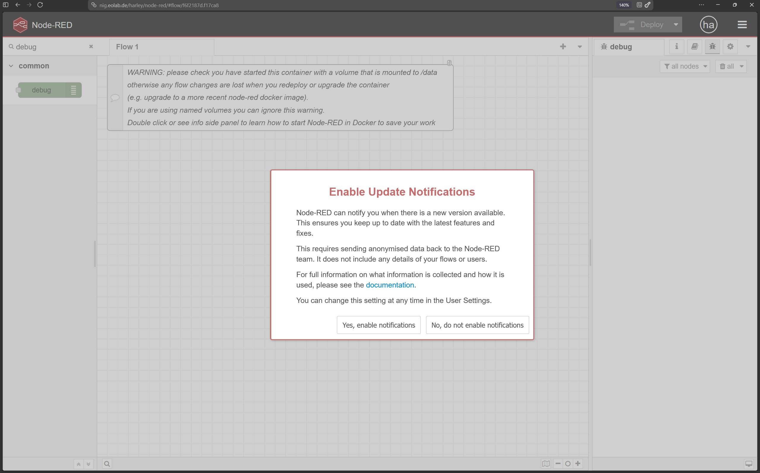
Node-RED editor. The interface contains the node palette, central flow workspace, and information and debug sidebar.

Continue the practical exercise from the previous chapter. In this section, you will configure Node-RED to subscribe to the MQTT topic used by your sensor and verify that the messages arrive correctly.

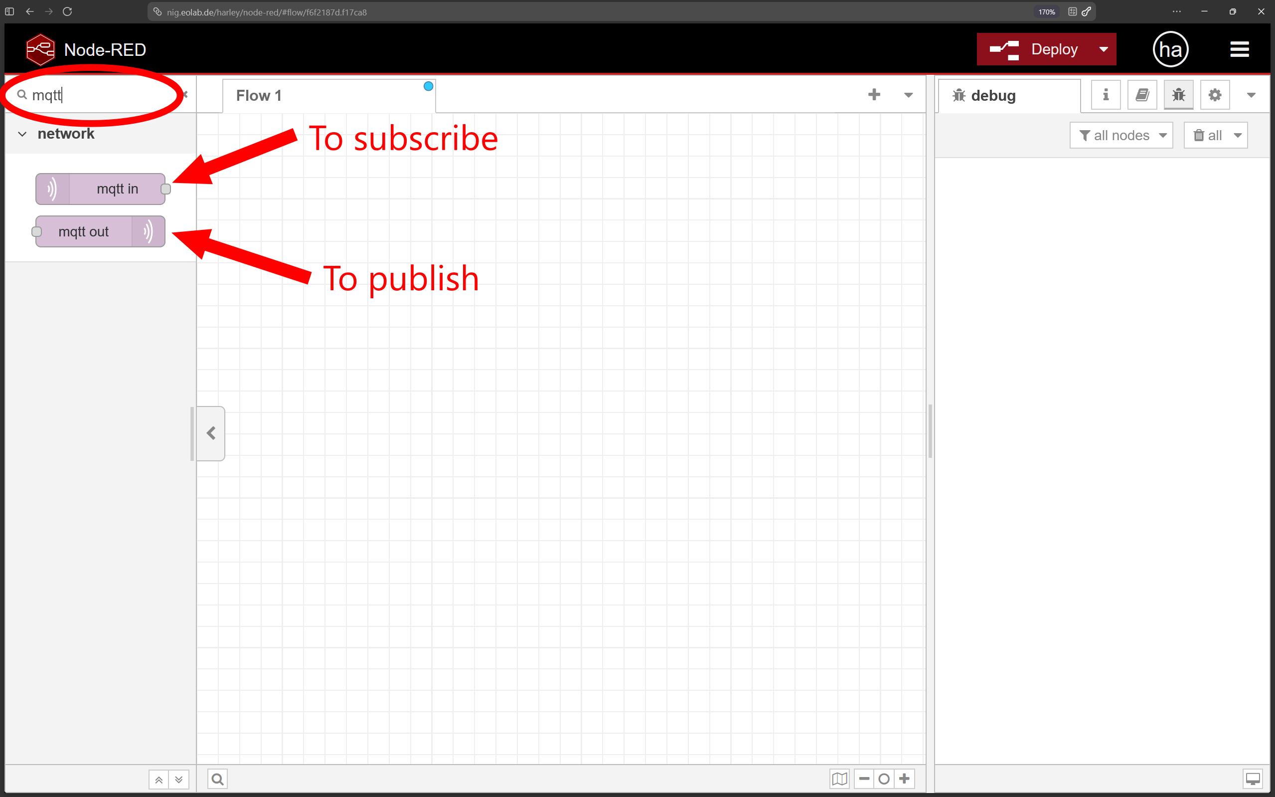
MQTT nodes in Node-RED. Use mqtt in to subscribe to a topic and mqtt out to publish messages.

• mqtt in: Connects to an MQTT broker and subscribes to messages from a specified topic.
• mqtt out: Connects to an MQTT broker and publishes messages to a specified topic.

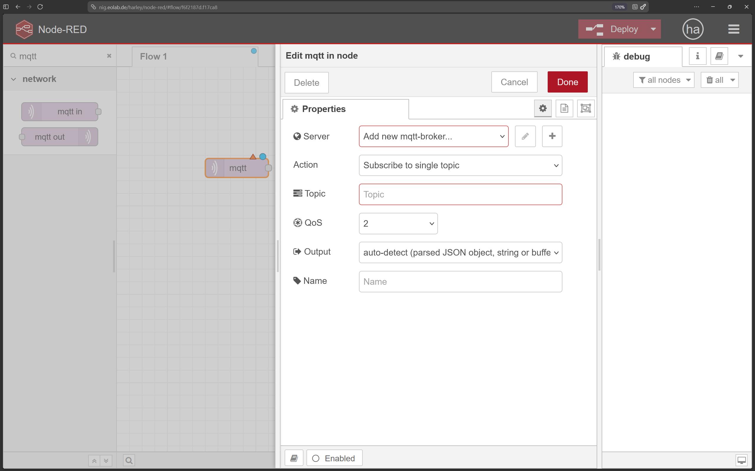
For this exercise, use an mqtt in node because Node-RED must receive the sensor data. Drag the node from the palette onto the central workspace, release it, and double-click it to open its configuration.

MQTT input node configuration. Open the node editor to select a broker, enter a topic, and configure the message output.

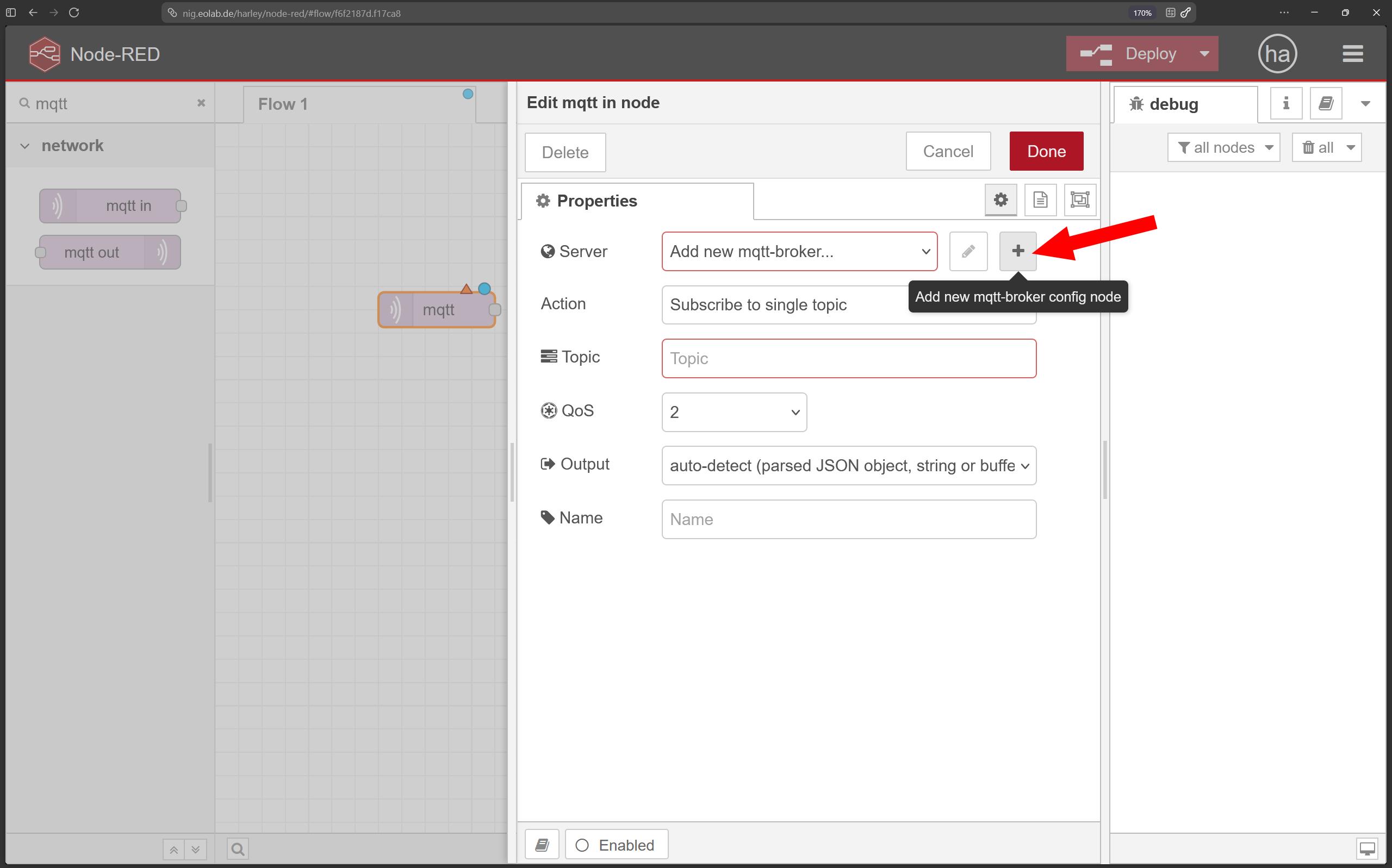
Adding an MQTT broker. Select the add-server button beside the broker field to create a broker connection.

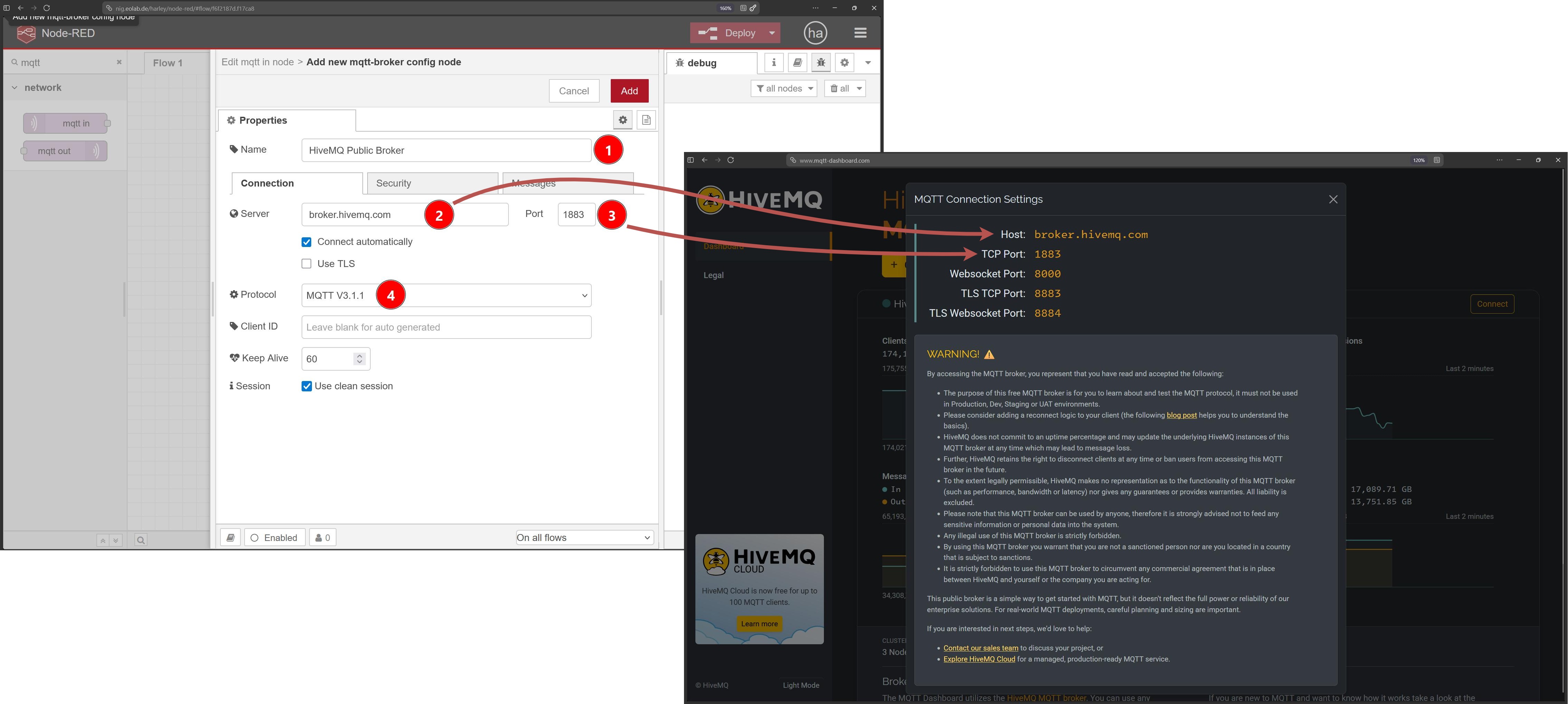
In the Server field, select the add-server button to create a broker configuration. Use the connection details provided on the HiveMQ Public Broker - MQTT Connection Settings page. Broker settings vary between providers, so always verify the hostname, port, security settings, and authentication requirements for the broker you are using. When the fields are complete, select Add.

MQTT broker settings. Enter the HiveMQ public broker connection details and select Add to save the configuration.

The new broker should now appear in the Server drop-down list. Broker configurations are shared across all MQTT nodes in your Node-RED instance, so the same saved connection can be reused in other flows. You may also create additional broker configurations when a project receives data from more than one broker.

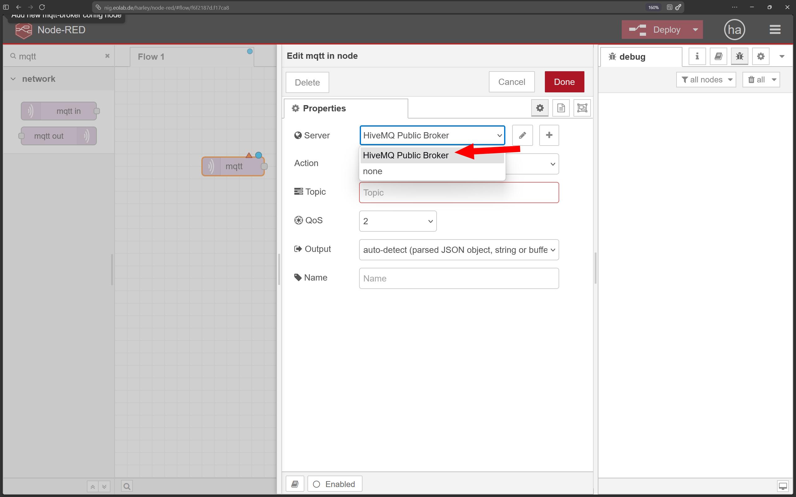Selecting the MQTT broker. Saved broker configurations are available to all MQTT nodes in the Node-RED instance.

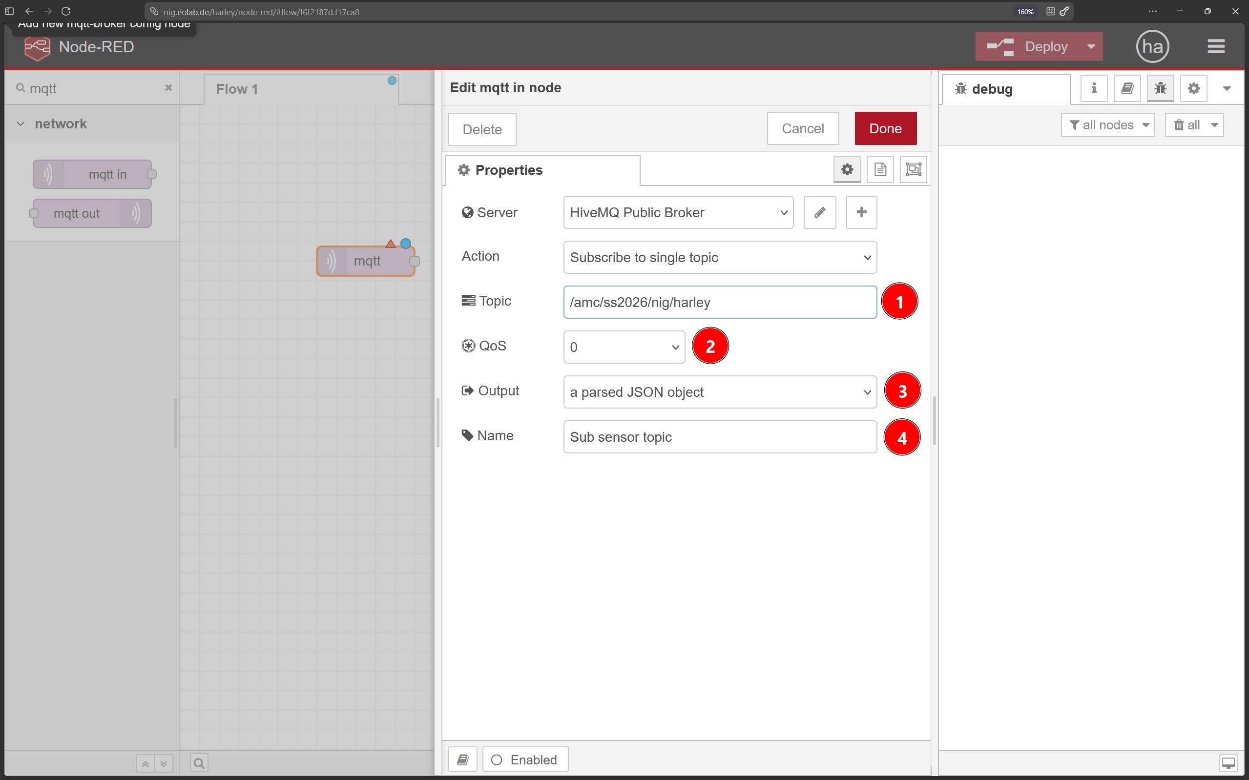Configured MQTT subscription. Specify the topic, use QoS 0, parse incoming messages as JSON objects, and assign the node a descriptive name.

Configure the mqtt in node as follows:

1. Topic: Enter the exact MQTT topic published by your sensor. Topic names are case-sensitive.
2. QoS: Select 0. For additional information about quality of service, refer to the MQTT chapter.
3. Output: Select the option that parses a valid JSON payload into a JavaScript object. The microcontroller used in this exercise publishes JSON, so this setting makes each sensor field directly available under msg.payload.
4. Name: Enter a descriptive label for the node, such as Subscribe to sensor data. This label does not affect the topic; it only helps identify the node in the flow.

MQTT transports payload bytes but does not enforce a particular data format. The publisher and subscriber must therefore agree on how the payload is structured. For example, three values could be sent as comma-separated text:

23, 456, 60

This representation is compact, but the subscriber must already know the position and meaning of each value. In this course, the sensor publishes JSON because each value can be identified by name:

{
  temperature_c: 23,
  co2_ppm: 456,
  relative_humidity: 60
}

JSON is easier to inspect and extend than a positional CSV-style payload. Its field names add message overhead, however, which can matter in battery-powered or bandwidth-constrained systems.

To verify the subscription, drag a Debug node onto the workspace and connect the output of the mqtt in node to its input. Select Deploy, then open the debug sidebar on the right.

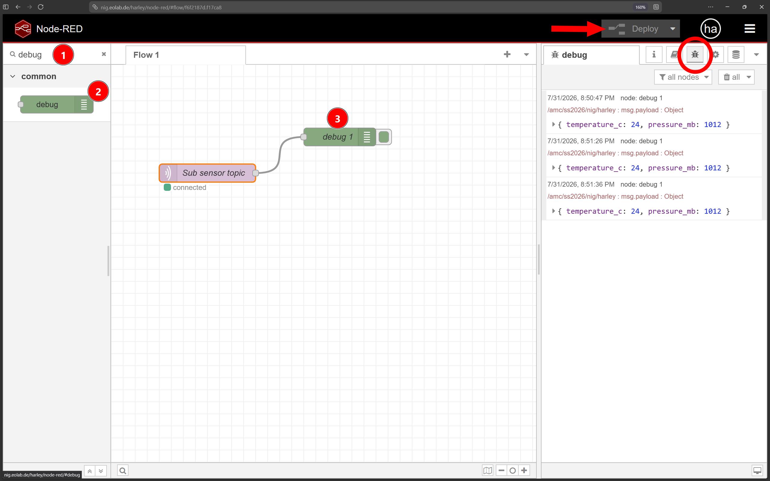Verifying MQTT messages. Connect a Debug node, deploy the flow, and confirm that subscribed messages appear in the debug sidebar.

Incoming messages should now appear in the debug sidebar. Confirm both the topic and the contents of msg.payload. If no messages appear, first verify that the configured topic exactly matches the topic used by the publisher. Also confirm that the publisher is active and that both clients are connected to the same broker.

For the concrete example used in this chapter, the payload has the following structure:

{
  temperature_c: 23,
  pressure_mb: 1013,
}

The temperature_c value comes from the DS18B20 sensor, and pressure_mb comes from the BMP280 sensor.

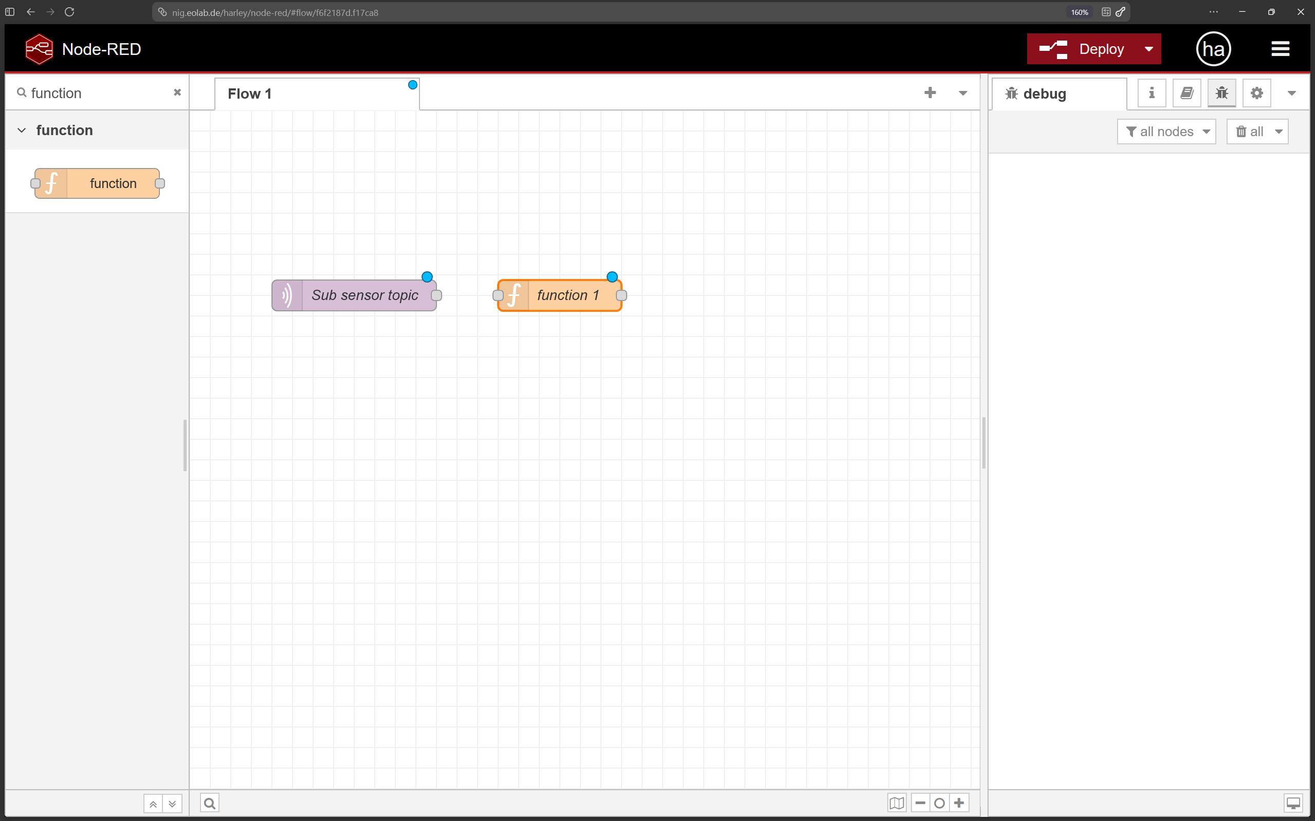Adding a Function node. Place a Function node after the MQTT input to validate and restructure the incoming sensor values.

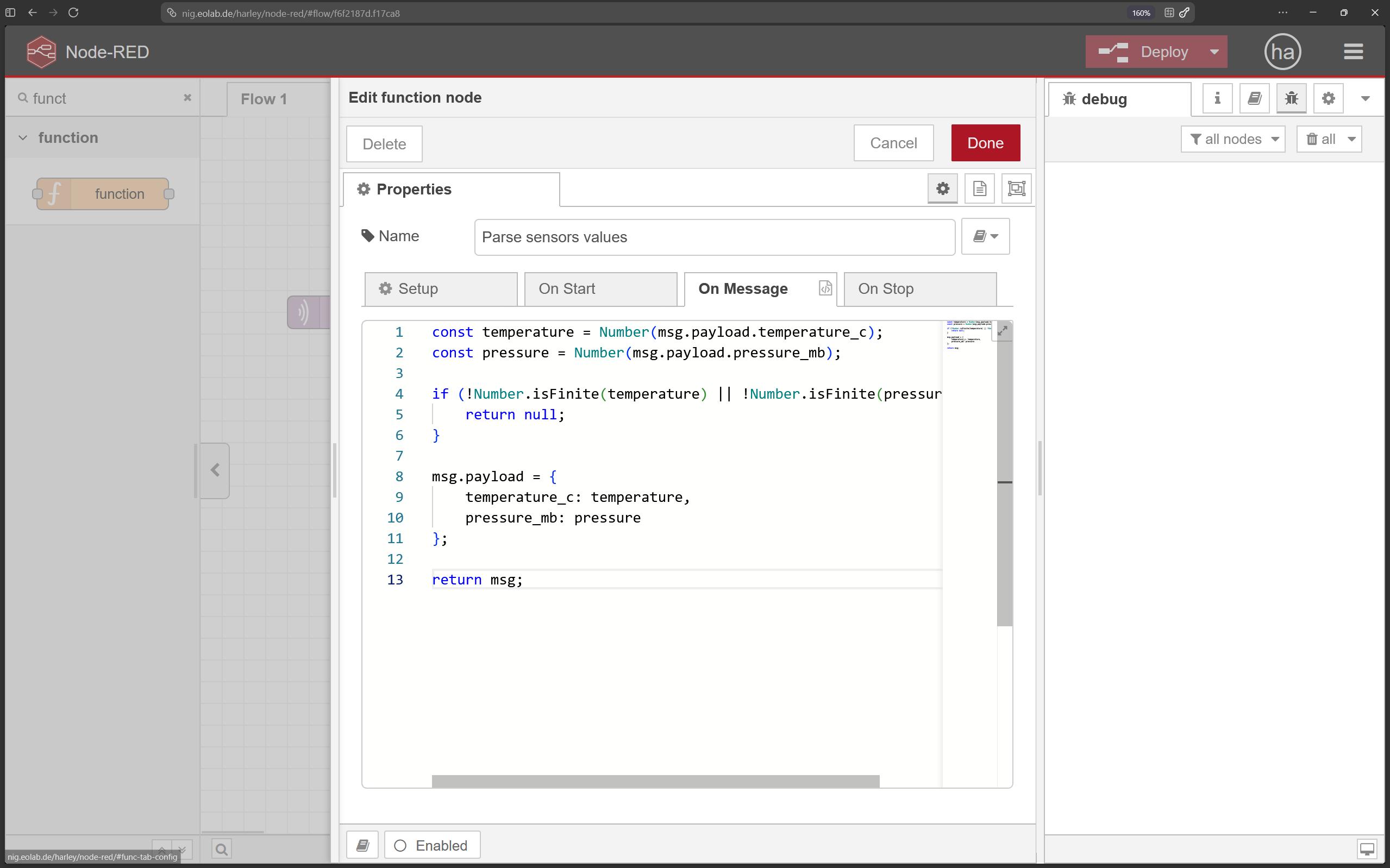
Before writing the values to InfluxDB, add a Function node after the mqtt in node. This function converts both fields to numbers and discards the message when either value is invalid. Paste the following JavaScript into the Function node:

const temperature = Number(msg.payload.temperature_c);
const pressure = Number(msg.payload.pressure_mb);

if (!Number.isFinite(temperature) || !Number.isFinite(pressure)) {
    return null;

}


msg.payload = {
    temperature_c: temperature,
    pressure_mb: pressure
};

return msg;

Function node logic. The JavaScript converts the sensor fields to numbers, rejects invalid values, and rebuilds msg.payload for storage.

Select Done, then connect the nodes in this order: mqtt in to function. You may keep the Debug node connected while testing.

The next step is to write the validated values to InfluxDB. InfluxDB nodes are not included in the default Node-RED installation, so searching the palette for influx may initially return no results. Install the community package that provides the required integration.

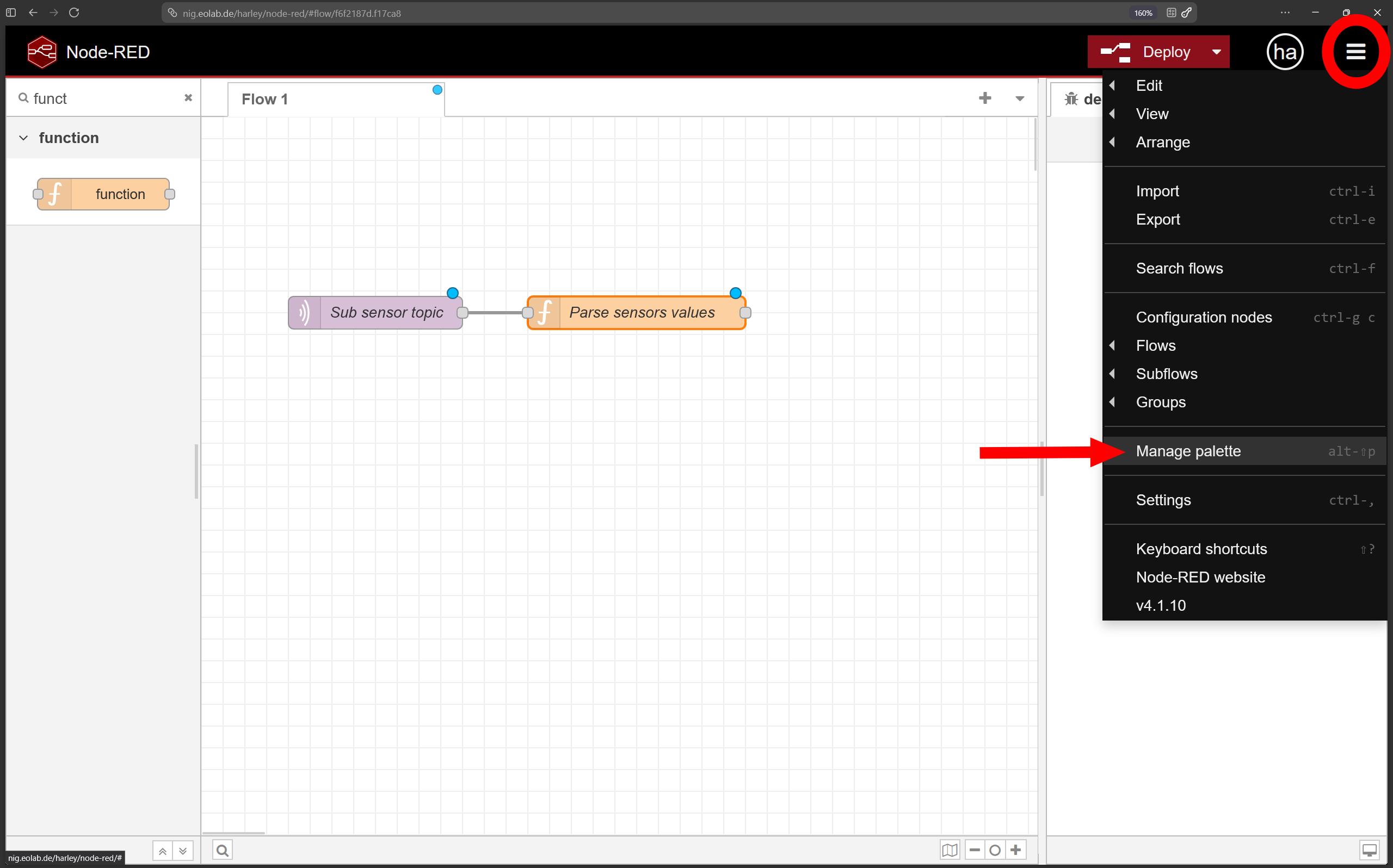
Open the main menu in the upper-right corner and select Manage palette.

Opening the palette manager. Use the main menu and select Manage palette to install additional Node-RED nodes.

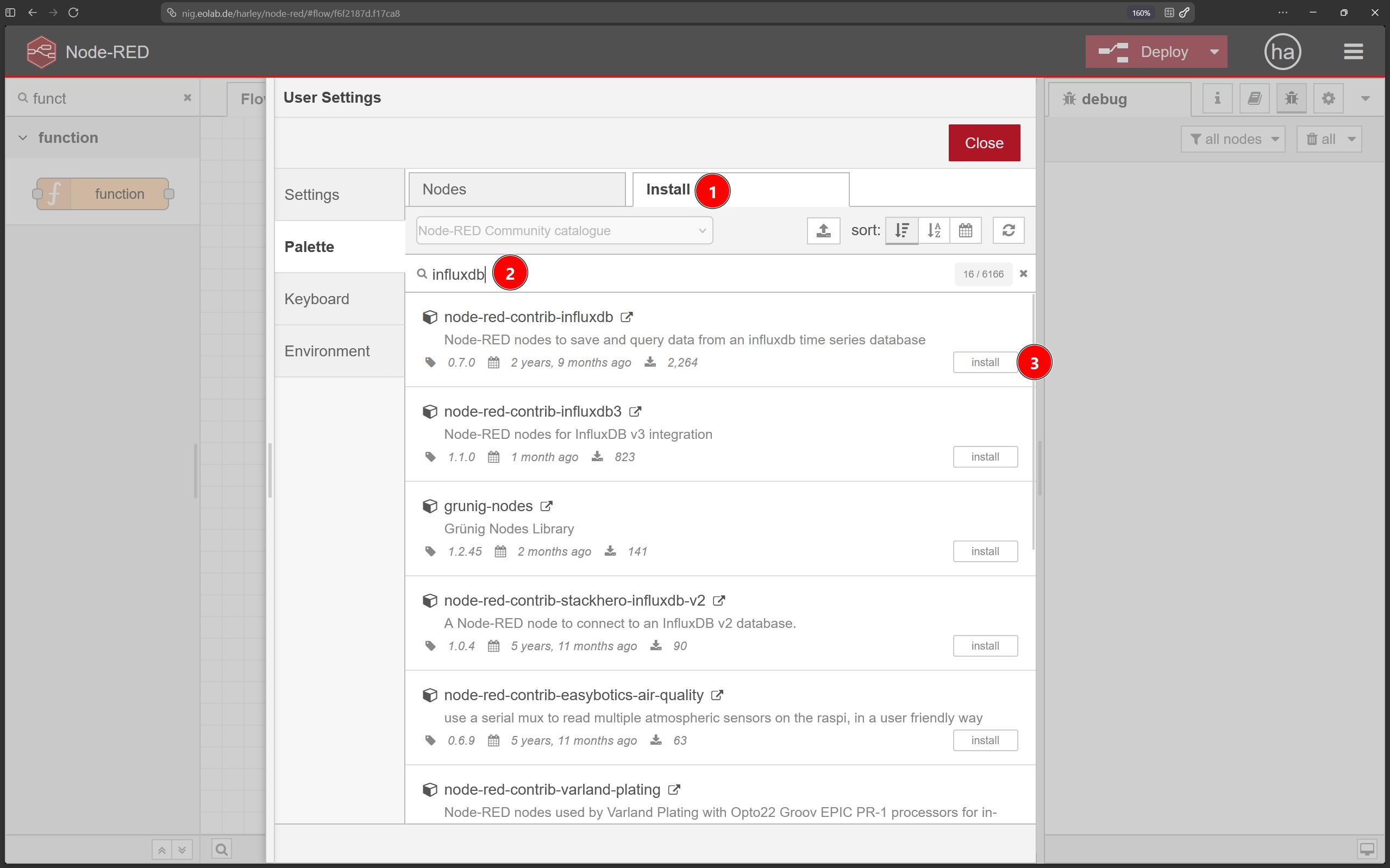
Open the Install tab, search for InfluxDB, locate the InfluxDB node package shown in the screenshot, and select Install. Confirm the installation if Node-RED displays a confirmation dialog.

Installing InfluxDB nodes. Search for the InfluxDB package in the Install tab and select Install.

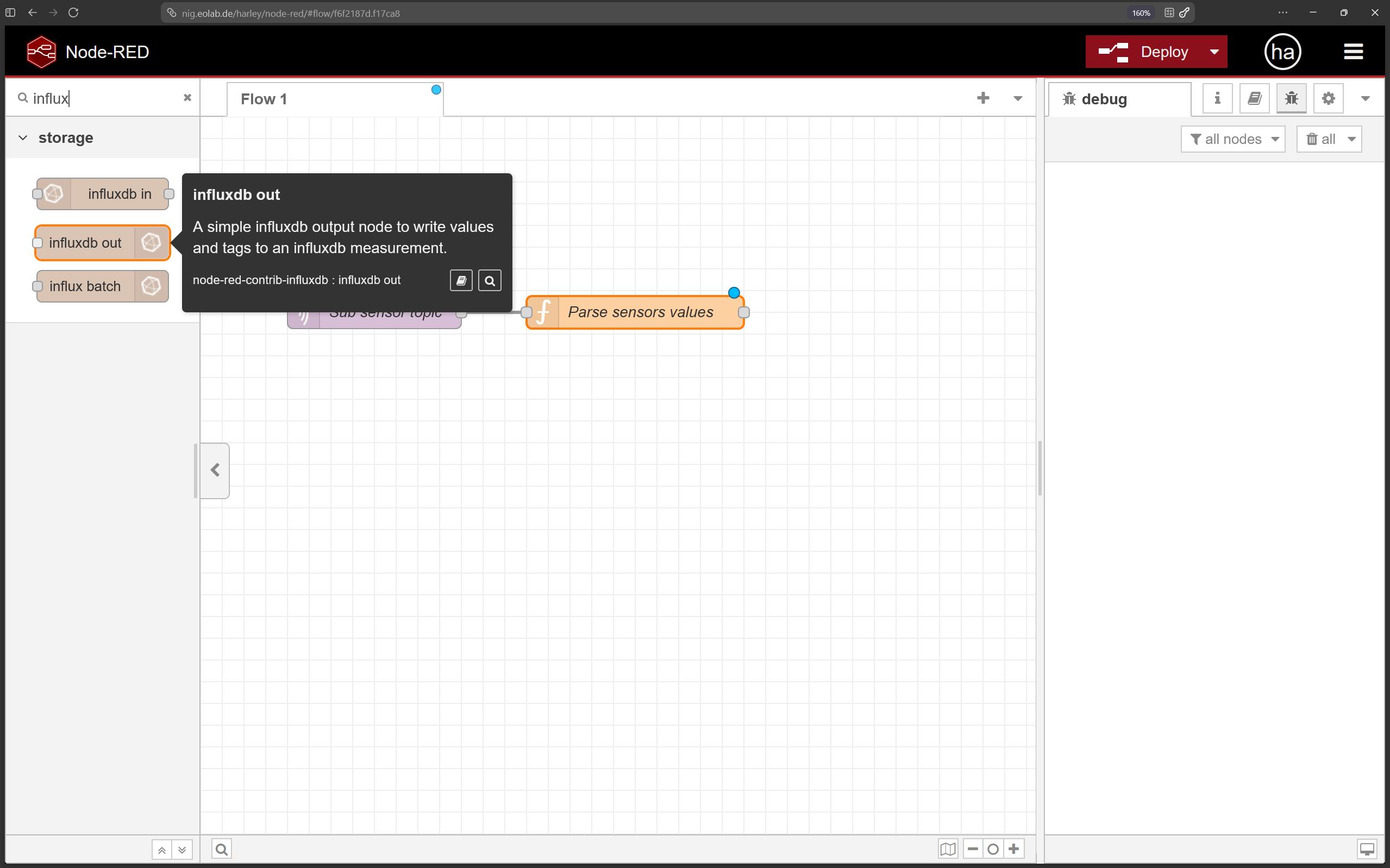
After the installation completes, close the palette manager and search the node palette for influx. The new InfluxDB input and output nodes should now be available.

InfluxDB nodes in the palette. After installation, the available InfluxDB input and output nodes appear in the Node-RED palette.

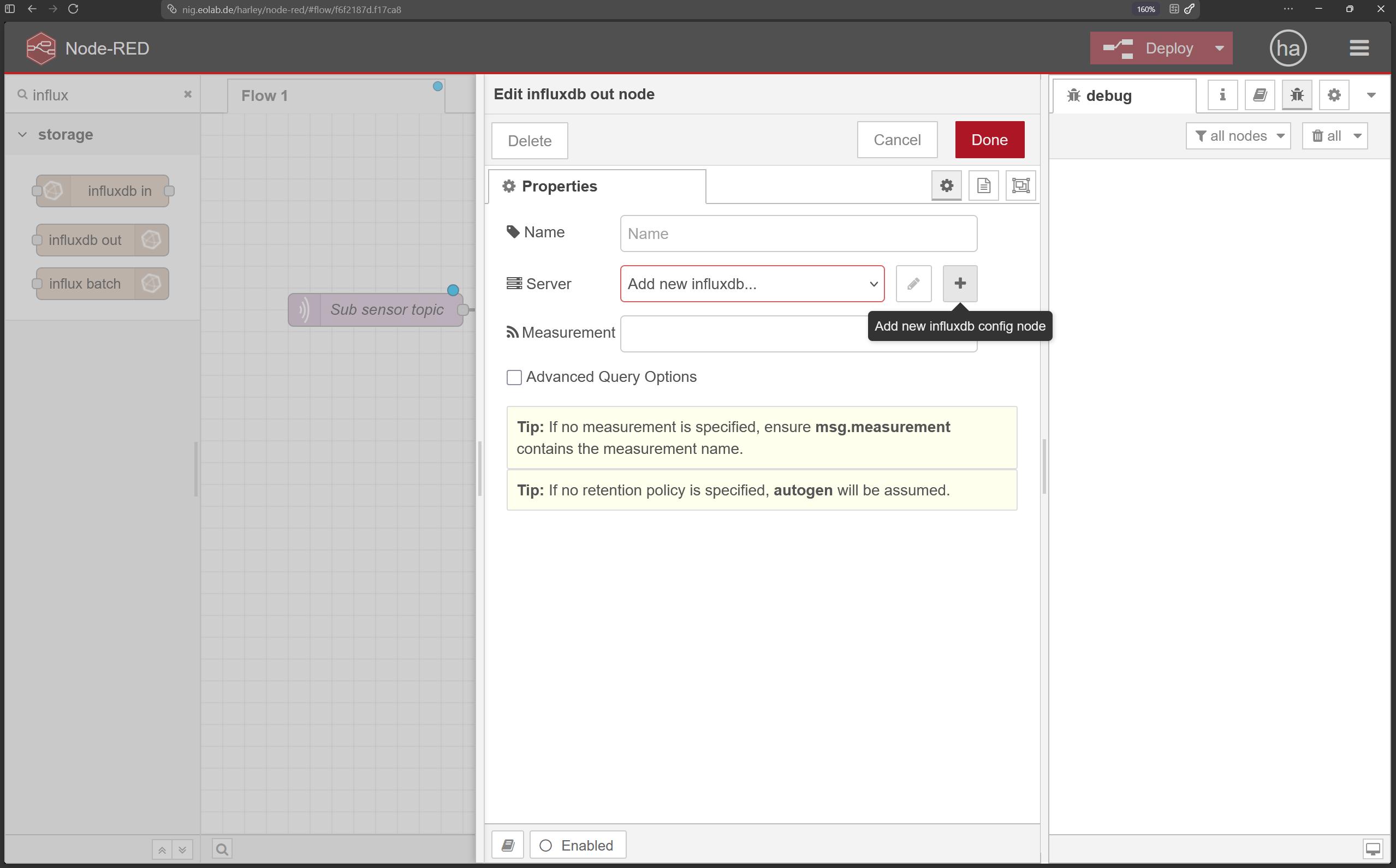
Adding an InfluxDB connection. Open the InfluxDB node editor and select the add-server button to create a database connection.

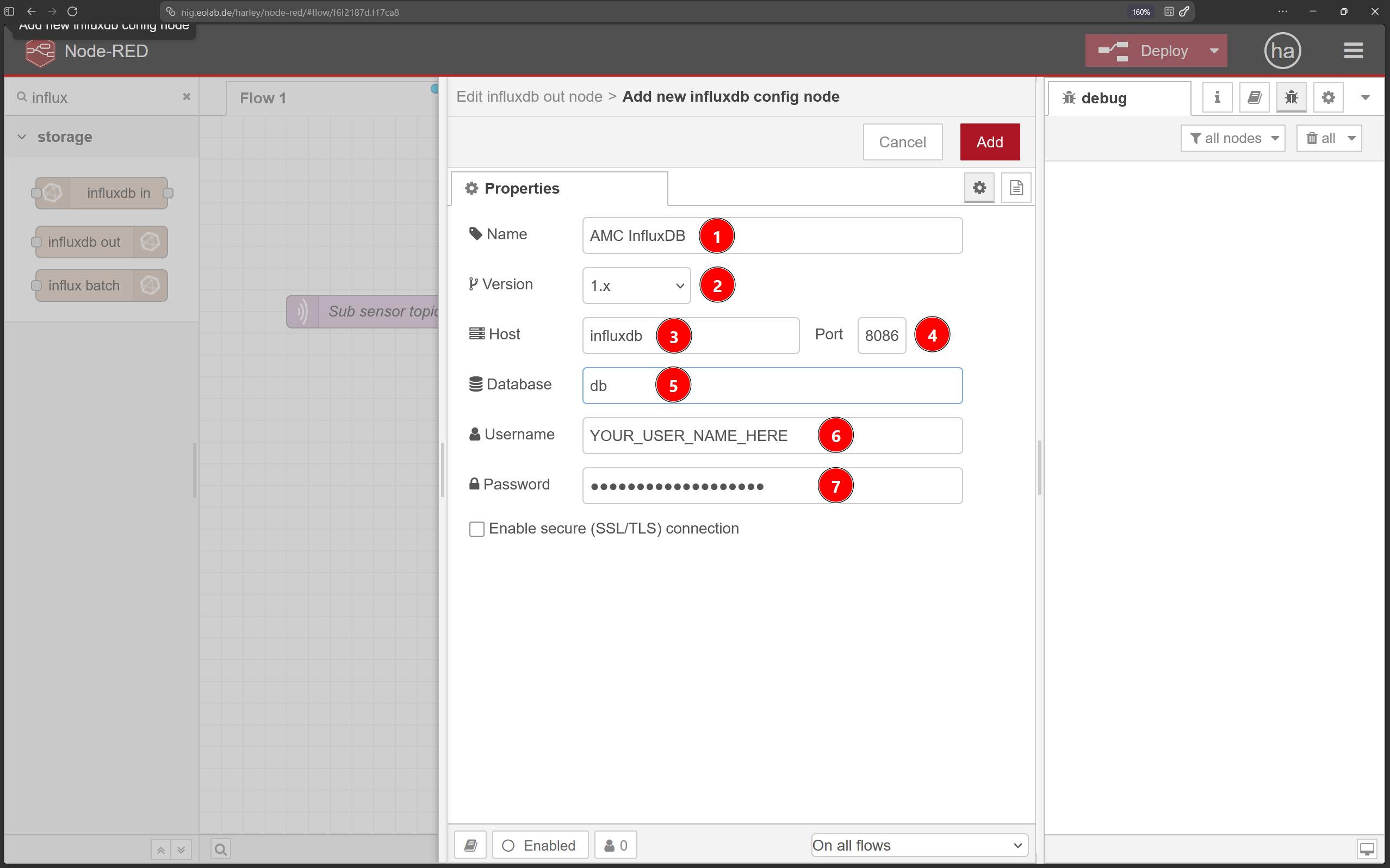
InfluxDB connection settings. Configure InfluxDB 1.x with host influxdb, port 8086, database db, and your AMC NIG credentials.

Drag an InfluxDB out node onto the workspace and open its configuration. Select the add-server button, then enter the following values: +1. Name: Enter a descriptive name for the connection, such as AMC InfluxDB. +2. Version: Select 1.x. +3. Host: Enter influxdb. This internal hostname is preconfigured by the AMC Teaching Team. +4. Port: Enter 8086. +5. Database: Enter db. This is the preconfigured database assigned to your environment. +6. Username: Enter the same username used to sign in to Node-RED. +7. Password: Enter the same password used to sign in to Node-RED.

Select Add to save the connection.

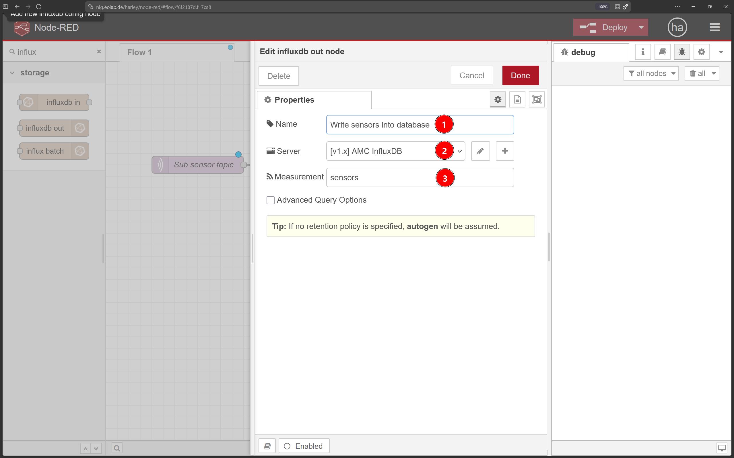
Back in the InfluxDB output-node configuration, select the connection you just created. Set the measurement to sensors and give the node a descriptive name. Both temperature_c and pressure_mb will be written as fields in this measurement. Remember the measurement name because Grafana will use it later when querying the stored data.

InfluxDB output node. Select the saved database connection and set the measurement name to sensors before writing sensor values.

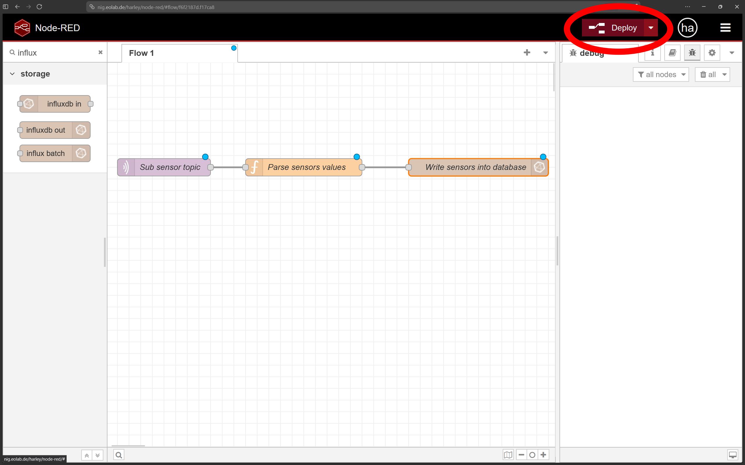
Connect the Function node to the InfluxDB output node. Check that the complete flow is connected correctly, then select Deploy to activate the subscription, validation, and database-writing steps.

Deploying the Node-RED flow. Select Deploy to activate the MQTT, processing, and InfluxDB changes.

As long as the MQTT publisher continues sending valid sensor readings, Node-RED will write new points to the sensors measurement in InfluxDB. If the database does not receive data, reconnect a Debug node after the Function node and verify that valid messages are reaching the InfluxDB output node.

---

InfluxDB

InfluxDB is important in Internet of Things applications because IoT devices typically generate large numbers of timestamped measurements. Sensors may repeatedly transmit values such as temperature, humidity, pressure, voltage, current, light intensity, or air quality. InfluxDB can store these measurements efficiently and preserve their chronological order, allowing changes and trends to be analyzed over time. Before the data is written to the database, it may be validated, converted into the correct units, filtered, or enriched with metadata. Once stored, the data can be queried to calculate averages, minimum and maximum values, rates of change, or measurements within a specific time interval.

Another important characteristic of InfluxDB is its ability to integrate with different data-processing, monitoring, and visualization tools. Data can be written to InfluxDB through its API, command-line tools, client libraries, or dedicated connectors available in platforms such as Node-RED. It can also provide data to visualization and monitoring systems such as Grafana. Measurements can be organized using tags and fields, which makes it possible to distinguish between devices, sensor types, locations, experiments, or operating conditions. This flexibility allows InfluxDB to support both small laboratory experiments and larger IoT monitoring systems.

In the context of the AMC course, InfluxDB is used as the database for storing sensor information received through the MQTT and Node-RED pipeline. Sensor devices publish their measurements to an MQTT broker, and Node-RED subscribes to the relevant topics. After receiving the messages, Node-RED processes the sensor values and converts them into the structure required by InfluxDB. This may include assigning a measurement name, separating values into fields, adding tags such as the device identifier or sensor location, and ensuring that every data point has an appropriate timestamp.

For our current exercise no direct configuration is required in the InfluxDB user interface for this exercise. Node-RED writes the data through the connection configured above, and Grafana reads it through the data source configured in the next section.

The processed information is then written from Node-RED into InfluxDB using dedicated database nodes. InfluxDB stores the measurements as time-series data, allowing students to retrieve values from specific time periods and compare the behavior of different sensors or devices. In the AMC course architecture, InfluxDB therefore represents the persistence layer of the IoT system. MQTT is responsible for transporting the sensor messages, Node-RED processes and routes them, and InfluxDB stores the resulting information for subsequent querying, analysis, and visualization.

---

Grafana

Grafana is important in Internet of Things applications because raw sensor measurements are often difficult to interpret when they are viewed only as individual numerical values. Grafana transforms these measurements into visual representations that make patterns, trends, anomalies, and changes easier to identify. For example, temperature measurements can be displayed as a time-series graph, current values can be shown using gauges, and sensor states can be represented using status panels. Users can also compare measurements from multiple sensors, select different time periods, and observe how the system behaves under different operating conditions.

Grafana is highly extensible and can integrate with many databases, cloud services, and monitoring platforms. It supports data sources such as InfluxDB, PostgreSQL, MySQL, Prometheus, Elasticsearch, and several cloud-based monitoring services. Dashboards can be extended with different panel types, variables, filters, annotations, and plugins. Grafana can also define alerts based on database queries. For example, an alert can be triggered when a temperature value exceeds a specified threshold or when a sensor stops reporting data. These integration capabilities make Grafana suitable for laboratory monitoring, industrial IoT systems, infrastructure supervision, and operational dashboards.

In the context of the AMC course, Grafana is used as the visualization layer of the IoT architecture. Sensor measurements are first transmitted through MQTT, processed by Node-RED, and stored in InfluxDB. Grafana then connects to InfluxDB as a data source and queries the stored measurements. Students can create dashboards that display current sensor readings, historical trends, minimum and maximum values, averages, and comparisons between different devices or sensor types.

The Grafana dashboards provide a visual interface through which students can evaluate the sensor data collected during an experiment. Time ranges can be adjusted to examine specific periods, while dashboard variables and filters can be used to select individual devices, measurements, or locations. In the AMC course workflow, Grafana completes the IoT data pipeline by converting the information stored in InfluxDB into understandable and interactive visualizations. The complete architecture therefore consists of sensors generating data, MQTT transporting the messages, Node-RED processing the information, InfluxDB storing the time-series measurements, and Grafana presenting the results for monitoring and analysis.

Open your personal Grafana instance using the URL below. Replace REPLACE_YOUR_USERNAME_HERE with your AMC NIG username, then sign in with your AMC NIG credentials.

https://nig.eolab.de/REPLACE_YOUR_USERNAME_HERE/grafana

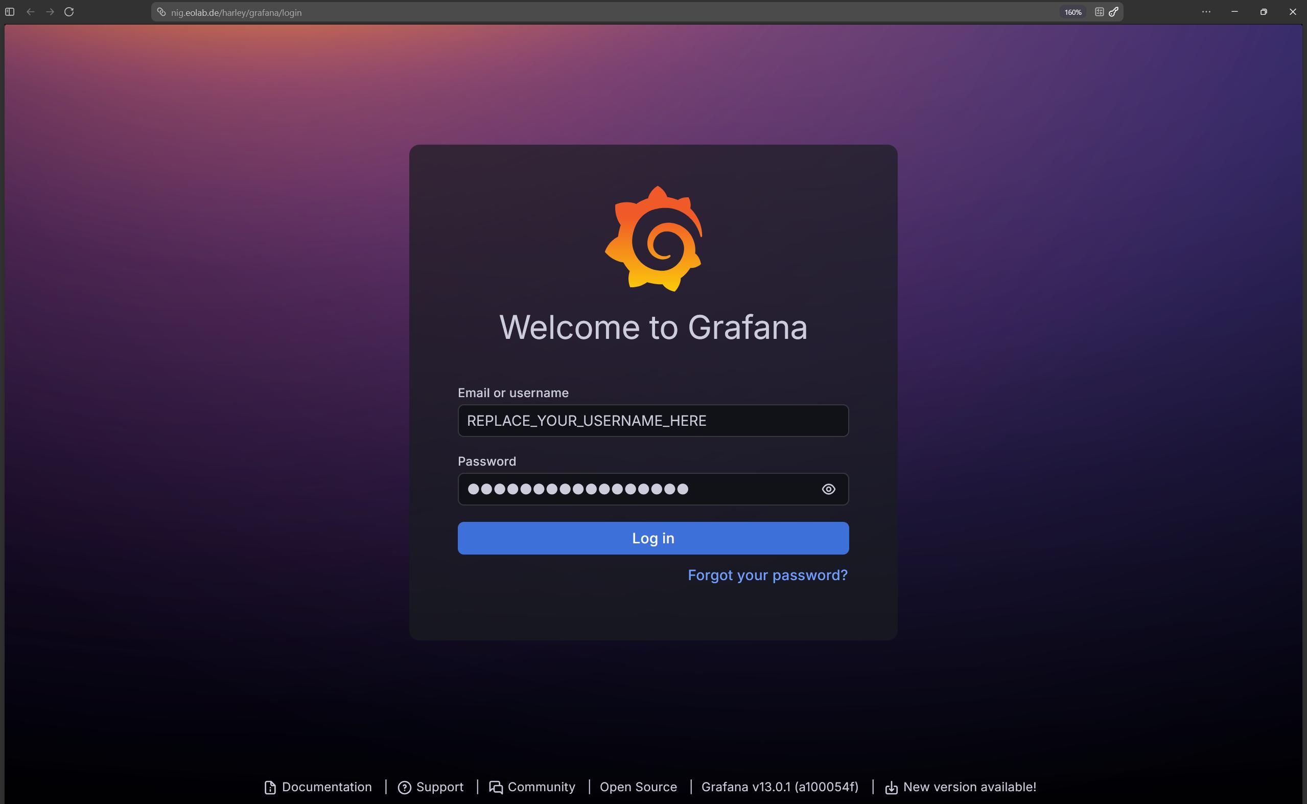Grafana sign-in page. Sign in with your AMC NIG account to access dashboards and data-source settings.

In Grafana, open Connections from the navigation menu and select Add new connection.

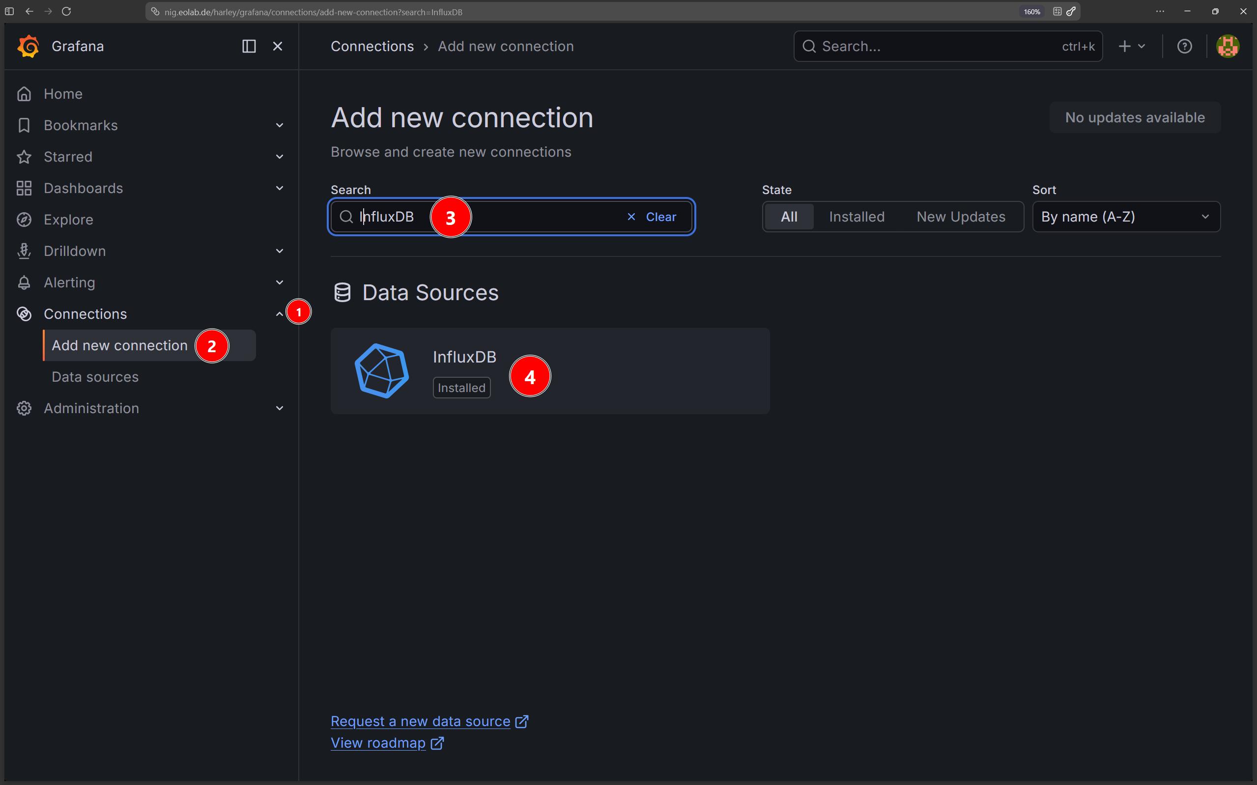Adding a Grafana connection. Open Connections and select Add new connection to configure InfluxDB as a data source.

Search for InfluxDB and select it from the list of available data sources.

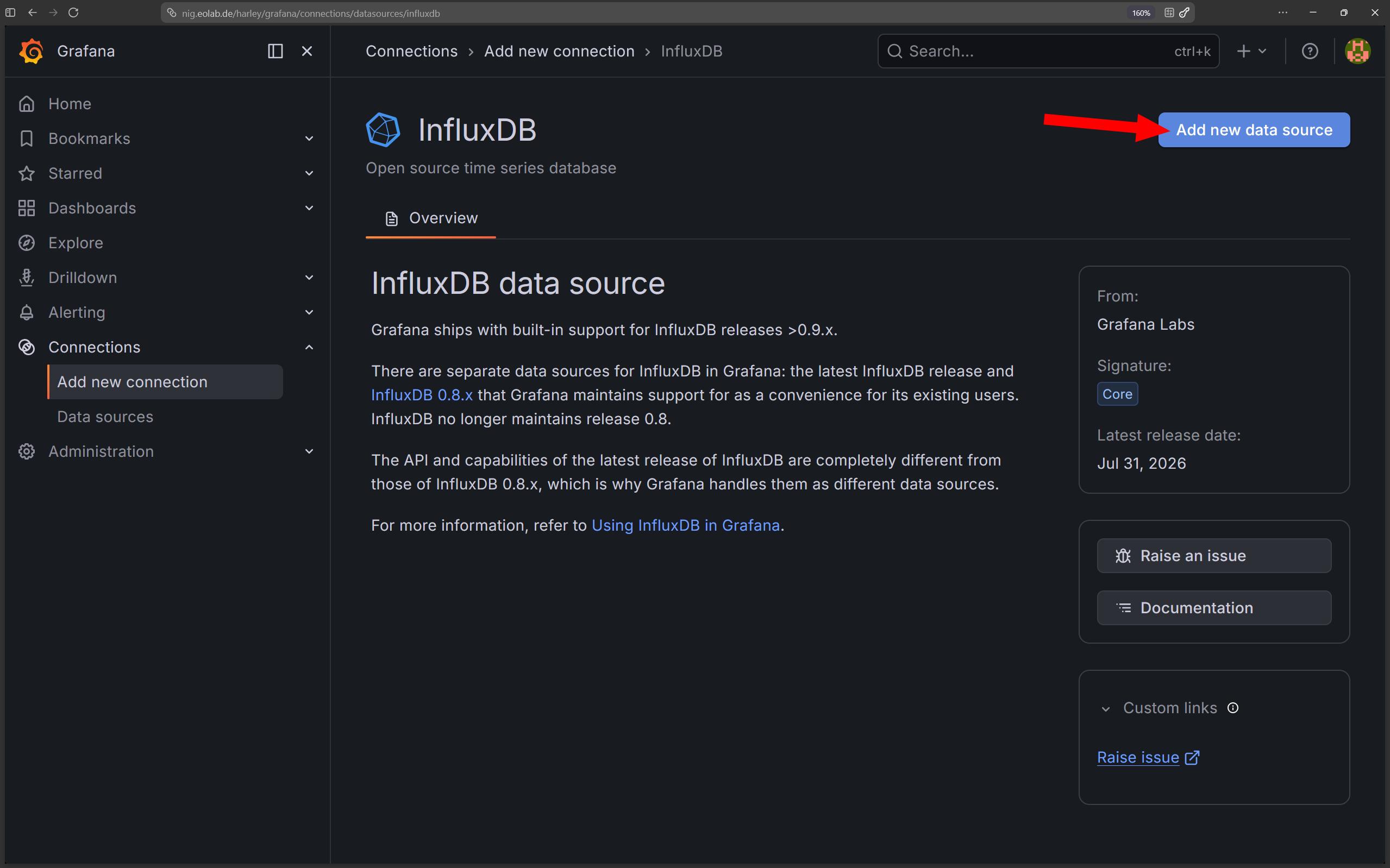Selecting the data source. Search for and select InfluxDB from Grafana’s available data-source integrations.

Create the InfluxDB data source using the connection values shown in the following screenshots. Use the same database name and AMC NIG credentials that you configured in Node-RED. Keep the query language and InfluxDB version consistent with the provided InfluxDB 1.x setup.

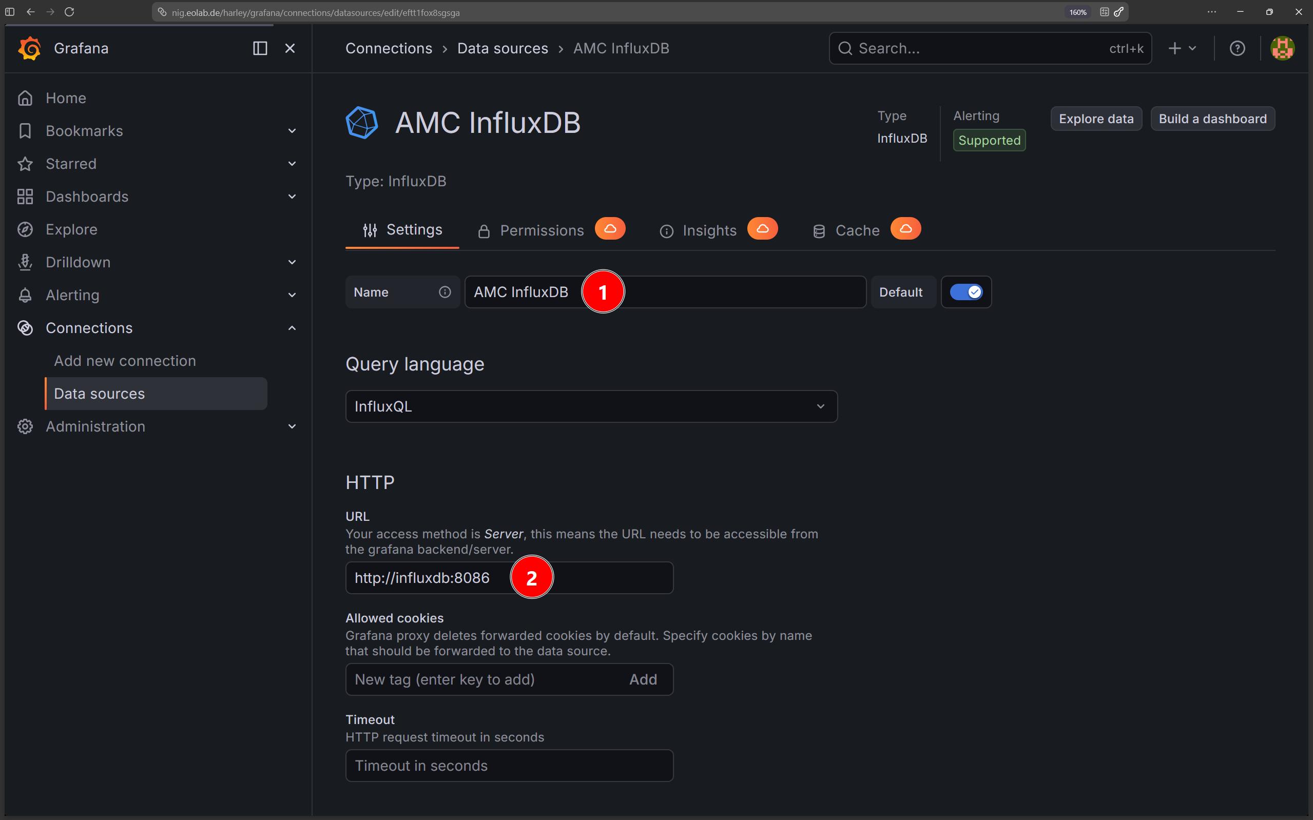InfluxDB data-source configuration, part 1. Enter the connection details required for Grafana to reach the course InfluxDB service.

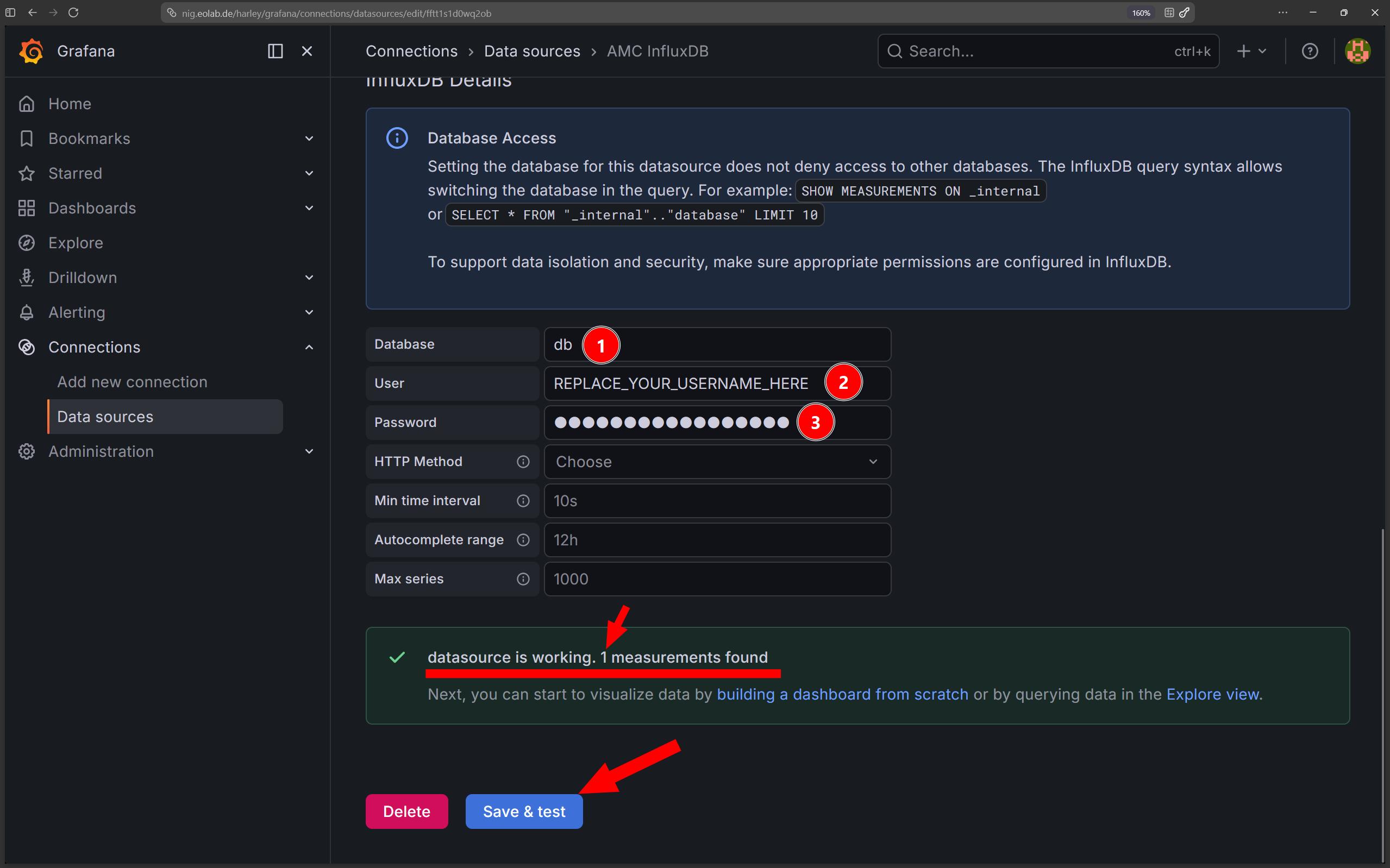
Complete the database and authentication fields. Then select Save & test. Continue only after Grafana confirms that the data-source connection is working.

InfluxDB data-source configuration, part 2. Complete the database and authentication settings, then save and test the connection.

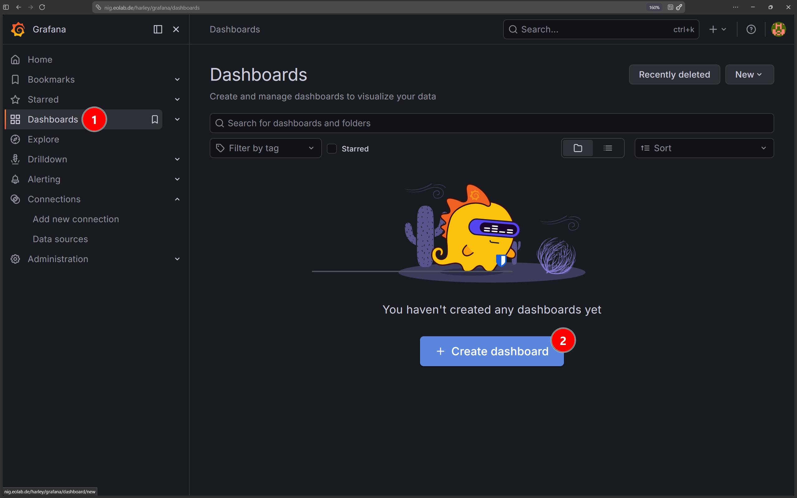
After the data source has been saved successfully, open Dashboards and create a new dashboard.

Creating a Grafana dashboard. Start a new dashboard to build visualizations from the stored sensor measurements.

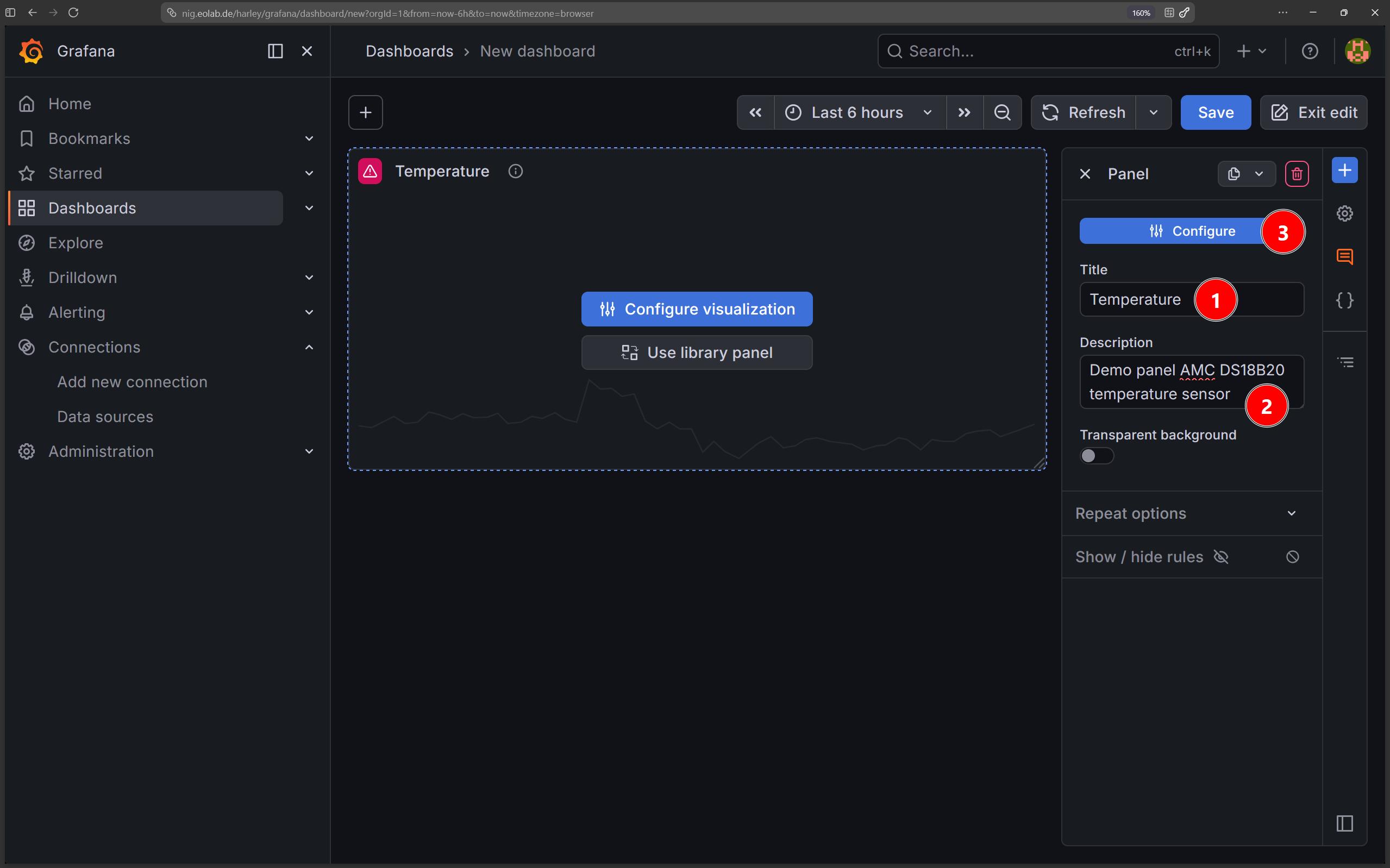
Select Add visualization to create the first panel. Grafana will open the panel editor, where you can define the data source, query, visualization, and panel options.

Adding a visualization. Add a panel to the new dashboard and open the panel editor.

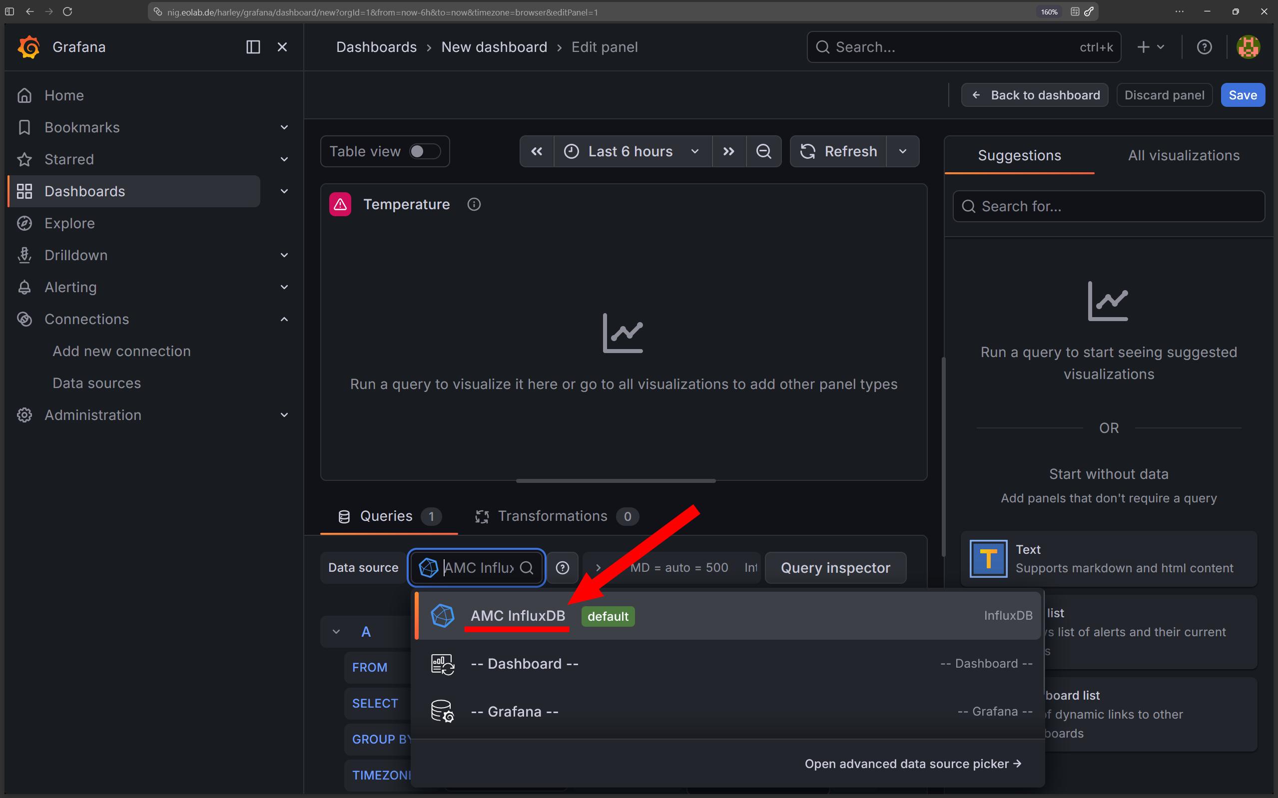
In the query section, confirm that the selected data source is the InfluxDB connection created in the previous step.

Checking the panel data source. Confirm that the panel query uses the InfluxDB connection configured in the previous steps.

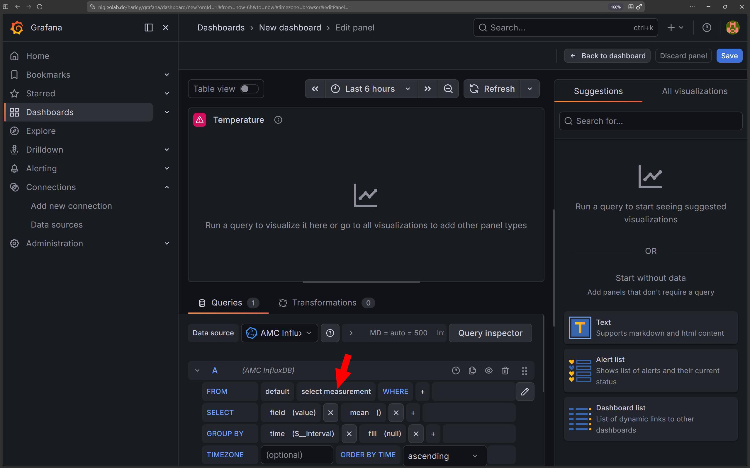
In the query builder, select the sensors measurement. This name must match the measurement configured in the Node-RED InfluxDB output node.

Selecting the measurement. In the panel query, choose the sensors measurement written by the Node-RED flow.

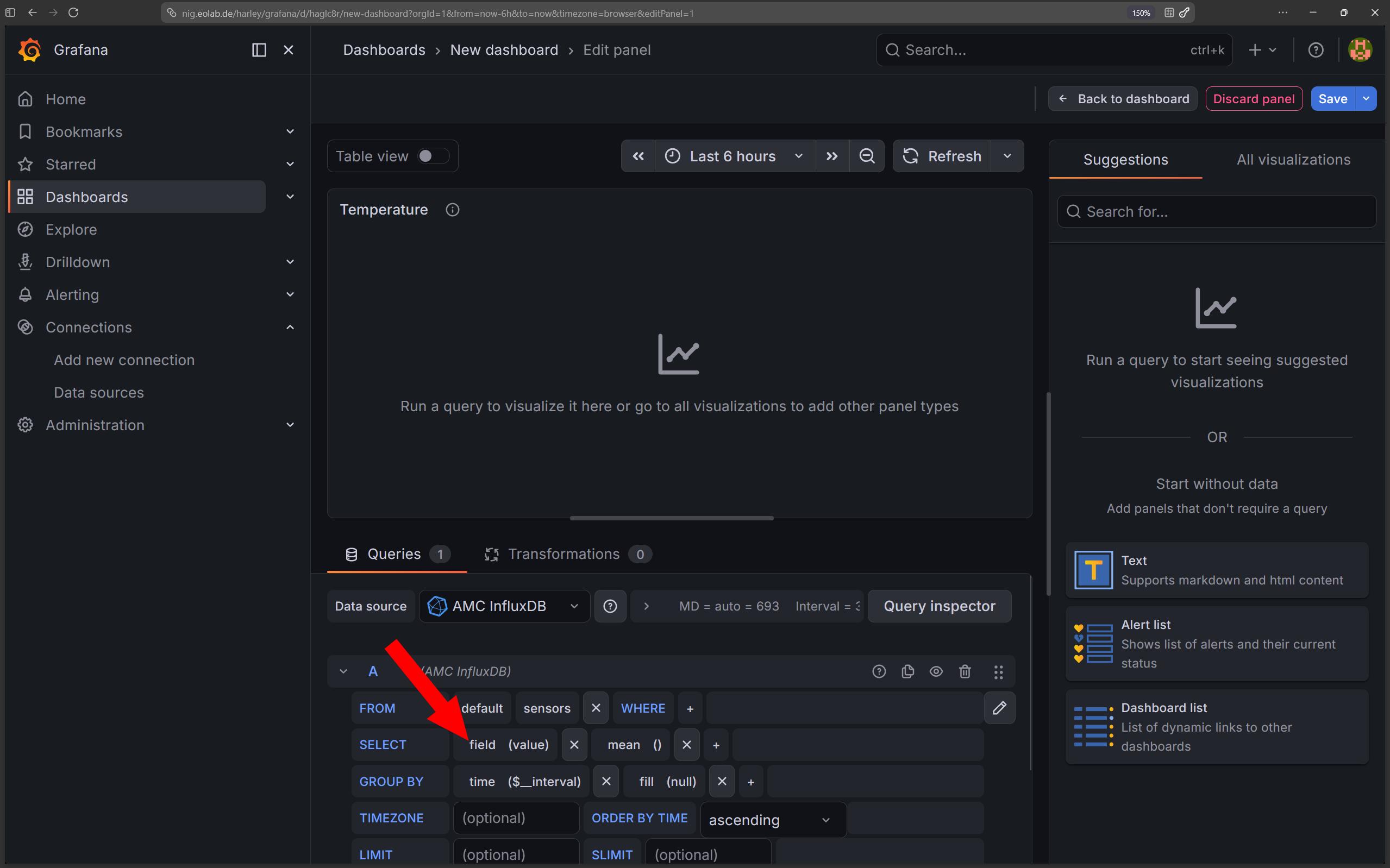
Open the field-selection menu to choose which sensor field the panel should display.

Selecting a measurement field. Open the field menu to choose which stored sensor value the panel should display.

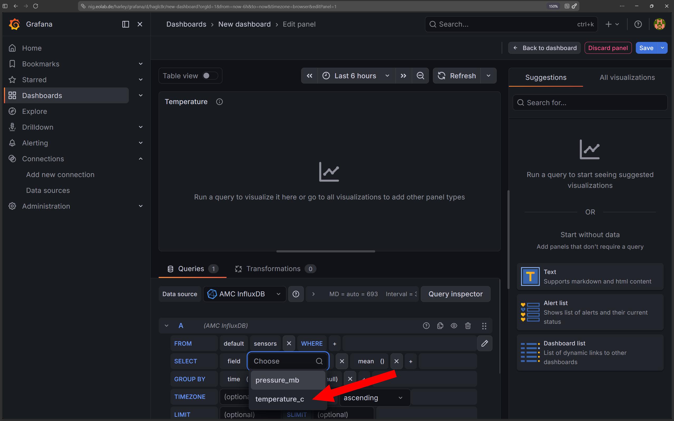
Select the temperature_c field. The panel preview should update as soon as Grafana retrieves matching data from InfluxDB.

Displaying temperature data. Select the temperature_c field to plot the stored temperature measurements.

The temperature values should now appear in the panel. If the panel shows no data, verify the selected data source, measurement, field, and time range. Also confirm that Node-RED is still writing current values to InfluxDB.

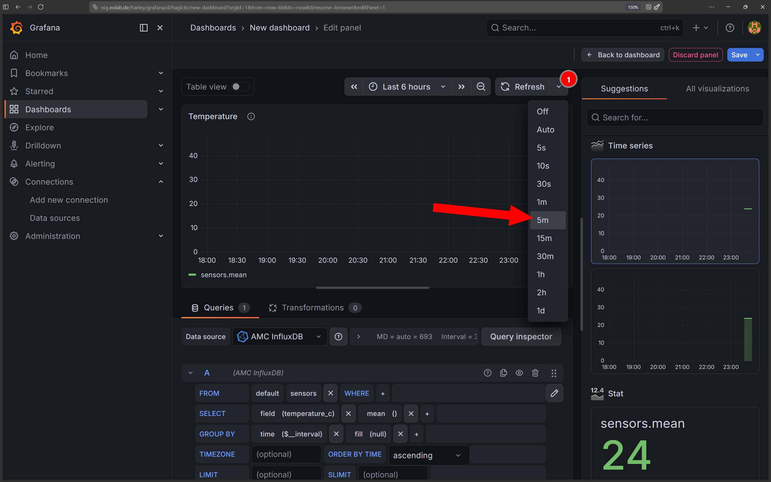
To update the dashboard automatically, open the refresh-interval menu and select 5m for a five-minute refresh interval.

Setting automatic refresh. Configure the dashboard to refresh its data every five minutes.

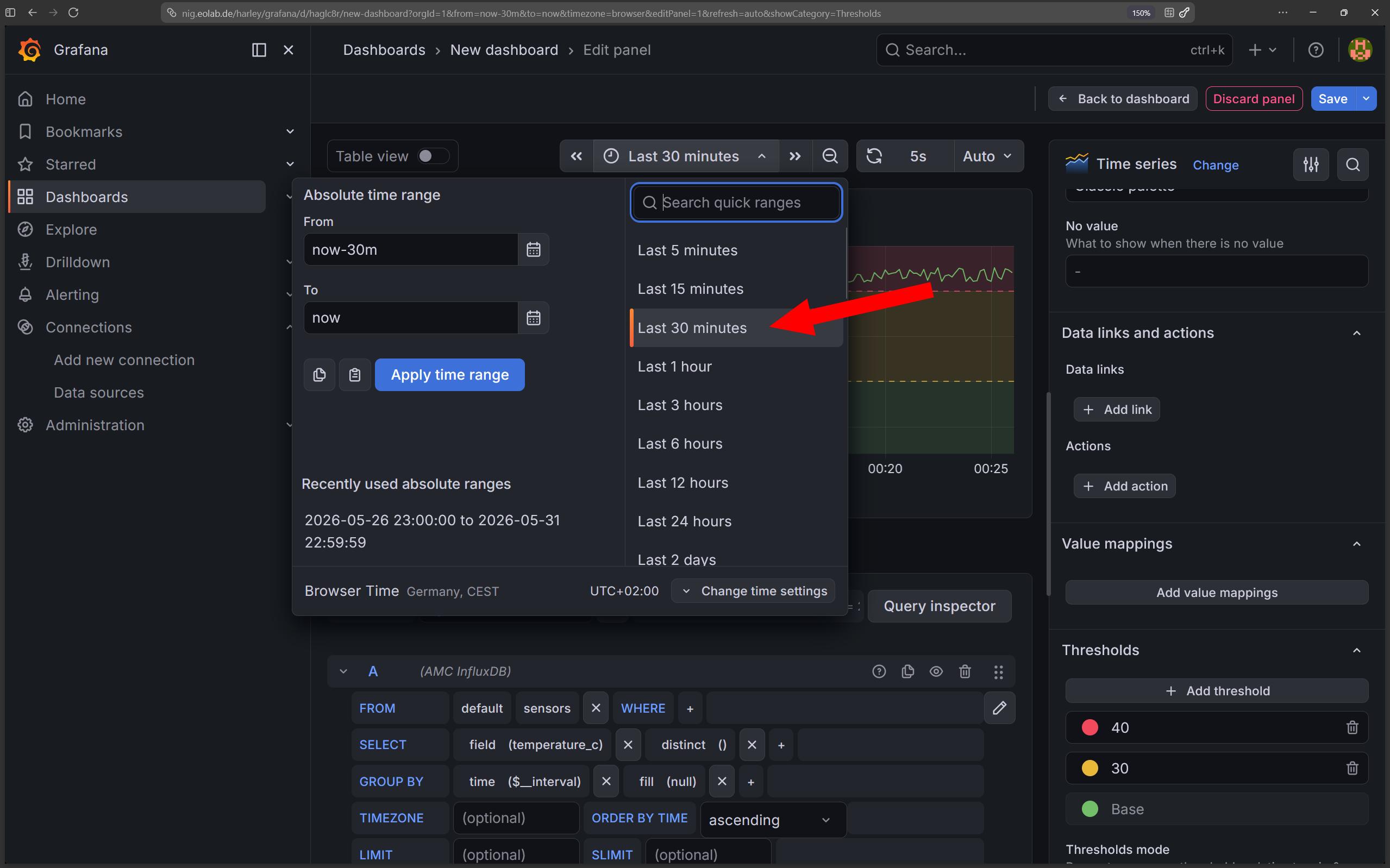
Next, open the time-range selector and choose Last 30 minutes so that the panel displays only recent measurements.

Setting the time range. Configure the dashboard to display measurements from the last 30 minutes.

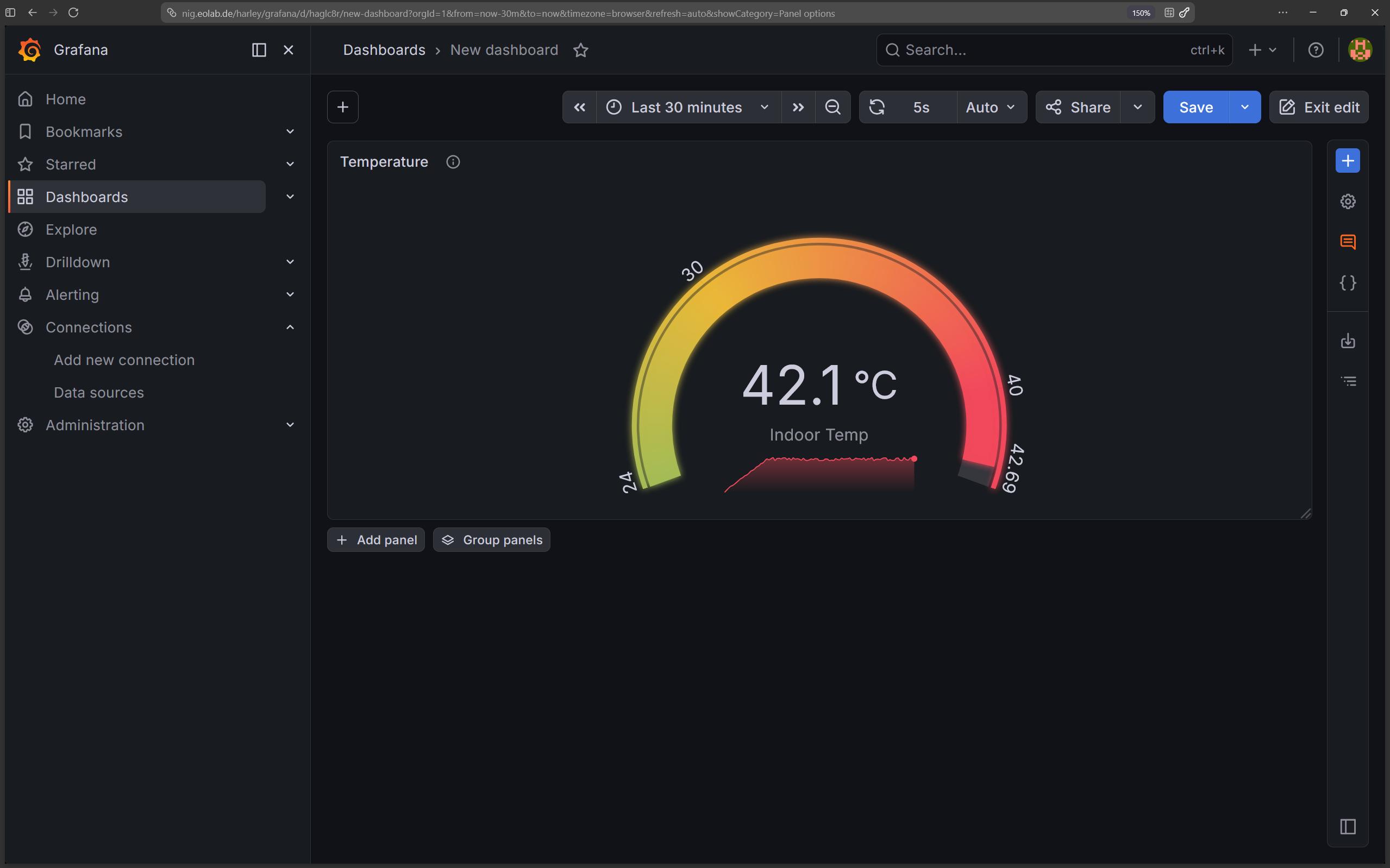
Save the dashboard and give it a descriptive name. You can then explore additional Grafana options such as panel titles, units, legends, thresholds, colors, and alternative visualization types.

Example temperature panel. The completed Grafana panel visualizes the stored temperature measurements over the selected time range.

Summary

The NIG stack brings together Node-RED, InfluxDB, and Grafana to form a complete IoT data pipeline. Each component has a clearly defined role within the architecture. Node-RED receives sensor messages, validates and transforms their contents, and routes the resulting data to the appropriate destination. InfluxDB stores these timestamped measurements as time-series data, while Grafana retrieves the stored values and presents them through interactive dashboards. Within the AMC environment, every student works with an isolated instance of the three services. Node-RED and Grafana are accessible through the internet, whereas InfluxDB remains the internal storage layer that connects processing with visualization.

The practical exercise developed this architecture from end to end. A sensor first publishes temperature and pressure values as a JSON message to an MQTT topic. Node-RED subscribes to that topic through an mqtt in node and converts the incoming payload into a JavaScript object. A Function node then converts the sensor values to numbers, rejects invalid messages, and restructures the payload for storage. The processed values are written to the sensors measurement in InfluxDB, where temperature_c and pressure_mb are preserved as fields associated with their timestamps. Grafana subsequently connects to the database, queries the measurement, and displays the selected field in a dashboard configured with an appropriate time range and automatic refresh interval.